Conway’s Game of Life Implemented in Clip Studio Paint

This is Conway’s Game of Life implemented using the popular drawing software Clip Studio Paint (CSP).

No, I’m not using the animation features in CSP, and I’m not drawing these pictures myself. Each frame is computed by Clip Studio Paint within the CSP file. The game advances every time we hit Save. How did I manage to squeeze this functionality out of a program that isn’t supposed to let us do anything more than edit images? Read on!

What is Conway’s Game of Life?

In case you haven’t heard of it, Conway’s Game of Life is a game that takes place on a two-dimensional grid. Each cell of the grid can either be dead or alive. When time advances by one step, each cell interacts with its neighbours —the eight cells that are vertically, horizontally, or diagonally adjacent to it—according to the following four rules:

1. If a live cell has fewer than two live neighbours, it dies (as if by underpopulation).
2. If a live cell has more than three live neighbours, it also dies (as if by overpopulation).
3. If a live cell has two or three live neighbours, it stays alive.
4. If a dead cell has exactly three live neighbours, it comes to life (as if by reproduction).

To put it more succinctly, we can condense these four rules into two:

1. A live cell stays alive if it has exactly two or three live neighbours; otherwise, it dies.
2. A dead cell comes alive if it has exactly three live neighbours; otherwise, it stays dead.

You can read all the words you want, but the best way to really understand Conway’s Game of Life is to play it yourself. There are plenty of websites (for example, this one) where you can do so. Go ahead; I’ll wait!

Manipulating pixel values in Clip Studio Paint

The Game of Life grid can be represented as a 2D image, where each pixel in the image is either black (dead) or white (alive). This is great because Clip Studio Paint, being an image manipulation program, provides us with a wealth of tools for modifying and combining pixel values.

Layers and layer blend modes

In CSP (among other image manipulation programs), a file contains mulitple layers, each representing a separate image. These layers are located in the Layer panel over to the side.

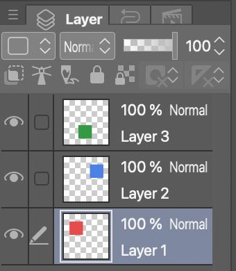
Layers can be moved and resized independently, in addition to being, well, layered on top of each other.

We can also combine the pixel values of two layers. In a (greyscale) digital image, each pixel has a value ranging from 0 (black) to 1 (white). If we stack two layers and set the blend mode of the top layer to Add, the values of the two layers will be added (and capped if it exceeds 1).

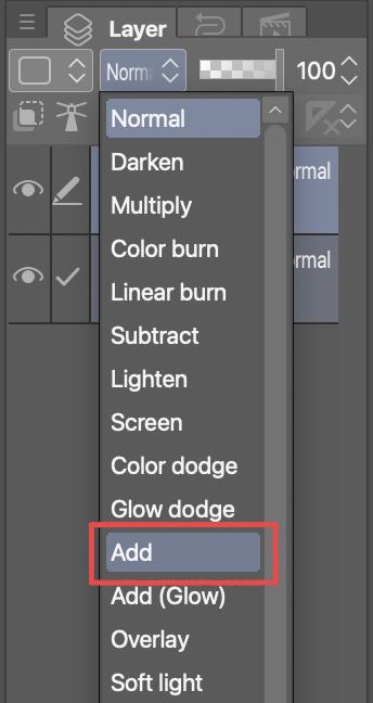
For example, I’ve filled these two layers with 50% grey (a value of 0.5). If I set one to Add and drag it over the other, they sum to white (a value of 1).

Tone Curves

Another pixel-value manipulation tool is the Tone Curve, found in the Layer > New Correction Layer menu. Adding a Tone Curve will create a new, special Tone Curve Layer.

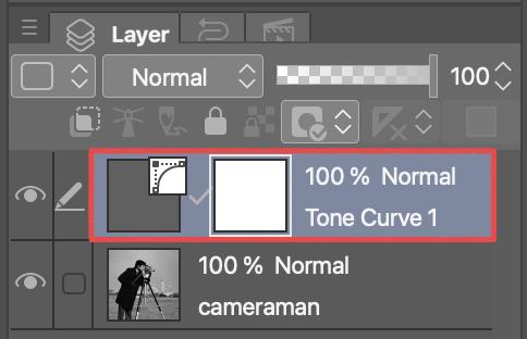
If we double-click on this Tone Curve layer, a graph appears. This graph defines a function mapping the input pixel value to an output value.

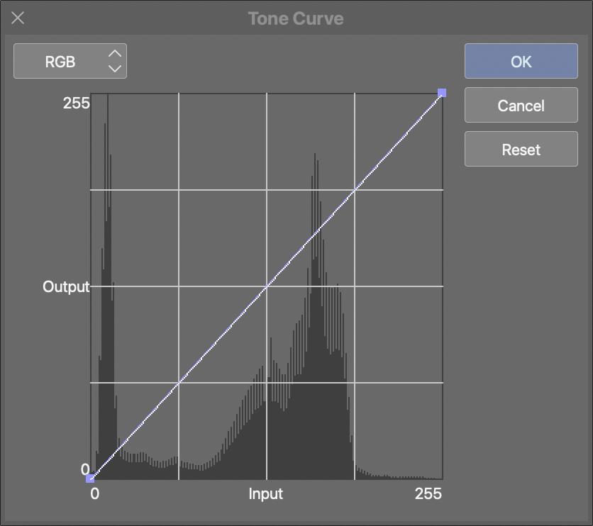
We can edit this function as we please. For instance, here I create a step function that sets all pixel values below 0.5 to black and the ones above 0.5 to white. This converts the image into a two-tone picture.

As another example, here I scale all pixel values by a factor of 0.5 by dragging the right endpoint down to the 50% mark. This darkens the entire image.

Calculating a step of the Game of Life

We now know how to add and scale pixel values. That’s all we need to implement the calculations necessary for running the Game of Life!

Let’s go back to our two rules:

1. A live cell stays alive if it has exactly two or three live neighbours; otherwise, it dies.
2. A dead cell comes alive if it has exactly three live neighbours; otherwise, it stays dead.

Representing “live” and “dead” by values of 1 (white) and 0 (black) respectively, this becomes:

1. A white pixel stays white if the sum of its neighbours’ values is between 2 and 3 inclusive; otherwise, it turns black.
2. A black pixel turns white if the sum of its neighbours’ values is exactly 3; otherwise, it stays black.

If we consider the pixel itself in the sum, we can actually condense this into a single rule:

1. A pixel should be white in the next step if the sum of its neighbours’ values, plus half of the pixel’s value, is between 2.5 and 3.5 inclusive. Otherwise, it should be black.

We can implement this calculation using Tone Curves and the Add blend mode. Let’s focus on a single pixel. We want to compute the sum of the values of the pixel’s neighbours, plus half its value.

First, we copy all eight neighbouring pixels onto separate layers and shift them on top of the middle pixel. This can be done by making eight copies of the overall image and shifting each of them in a different direction by one pixel.

We set the blend modes of the new layers to Add, as well as halving the value of the middle pixel using a Tone Curve layer.

Hmm, it’s all white. We forgot to consider the fact that pixel values are capped at 1—too small to hold the entire sum. Fortunately, this can easily be fixed by scaling down the pixel values. Using Tone Curves, we divide each pixel value by 5 before adding it to the total. Note that we select the Clip to Layer Below option on each Tone Curve to ensure it applies only to the layer directly below it.

All right! The value of the middle pixel should now equal the sum of the values of its neighbours, plus half its original value, divided by 5. The pixel should become white if its value is between 2.5 / 5 = 0.5 and 3.5 / 5 = 0.7, and black otherwise. We can make this change by adding a final Tone Curve representing a step function. This Tone Curve outputs 1 if the input is between 0.5 and 0.7 (with a bit of leeway on either side), and 0 otherwise.

We did it! We calculated the next state of the pixel! Of course, we did have to copy and shift the image eight times. How tedious. There must be a faster way to do it…

A faster way to do it: the Create File Object command

Let’s switch gears and talk about the Create File Object command, found under the File > Import menu. Create File Object allows you to import another CSP file into your current file. If the external file is changed and saved, the imported image updates accordingly.

This may lead you to wonder: can you import a file into itself?

Yes, you can! If you do that, the entire image will be copied and placed within itself every time you save the file. (This makes for some very fun Inception-esque effects.)

Now we don’t need to copy the image manually. Instead, we import the file into itself nine times, shifting eight of those import layers in different directions by one pixel. We change the layer blend modes to Add and apply Tone Curves as before, then hit Save. The game moves forward automatically.

And there we have it! Conway’s Game of Life, implemented in Clip Studio Paint. Here’s a link to the CSP file in case you want to try it out yourself (it’s been tested with CSP Version 1.13.2).

Conway’s Game of Life in Photoshop?

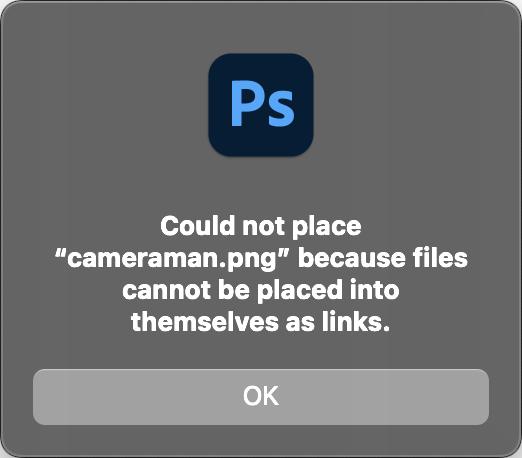
Can the same method be used to implement the Game of Life in the better-known image manipulation program Adobe Photoshop? Not exactly, because Photoshop, being the inferior software, does not allow you to import files into themselves.

However, Photoshop does have one thing that CSP lacks: the Custom filter, found in Filter > Other. This filter lets you specify the value of a pixel as a weighted sum of the values of surrounding pixels.

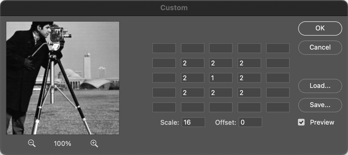
This eliminates the need for copying and shifting layers! We can implement a step of the Game of Life via a single Custom filter followed by a Tone Curve. It seems, though, that I’ve been beaten to the punch here—see Kelly Egan’s site for a Photoshop Auto Action that implements just this (except with a Gradient Map instead of a Tone Curve, which does something similar).

Clip Studio Paint is Accidentally Turing-Complete

One last fact for you to mull over: Conway’s Game of Life is Turing-complete—roughly speaking, this implies it can be used to simulate a general-purpose computer. Since CSP can simulate the Game of Life, it is also Turing-complete, so can also simulate a computer. This means that theoretically, with a large enough canvas, you would be able to run Clip Studio Paint…in Clip Studio Paint.

See you next time!